Google voice search: faster and more accurate
September 24, 2015
Posted by Haşim Sak, Andrew Senior, Kanishka Rao, Françoise Beaufays and Johan Schalkwyk – Google Speech Team
Back in 2012, we announced that Google voice search had taken a new turn by adopting Deep Neural Networks (DNNs) as the core technology used to model the sounds of a language. These replaced the 30-year old standard in the industry: the Gaussian Mixture Model (GMM). DNNs were better able to assess which sound a user is producing at every instant in time, and with this they delivered greatly increased speech recognition accuracy.
Today, we’re happy to announce we built even better neural network acoustic models using Connectionist Temporal Classification (CTC) and sequence discriminative training techniques. These models are a special extension of recurrent neural networks (RNNs) that are more accurate, especially in noisy environments, and they are blazingly fast!
In a traditional speech recognizer, the waveform spoken by a user is split into small consecutive slices or “frames” of 10 milliseconds of audio. Each frame is analyzed for its frequency content, and the resulting feature vector is passed through an acoustic model such as a DNN that outputs a probability distribution over all the phonemes (sounds) in the model. A Hidden Markov Model (HMM) helps to impose some temporal structure on this sequence of probability distributions. This is then combined with other knowledge sources such as a Pronunciation Model that links sequences of sounds to valid words in the target language and a Language Model that expresses how likely given word sequences are in that language. The recognizer then reconciles all this information to determine the sentence the user is speaking. If the user speaks the word “museum” for example - /m j u z i @ m/ in phonetic notation - it may be hard to tell where the /j/ sound ends and where the /u/ starts, but in truth the recognizer doesn’t care where exactly that transition happens: All it cares about is that these sounds were spoken.
Our improved acoustic models rely on Recurrent Neural Networks (RNN). RNNs have feedback loops in their topology, allowing them to model temporal dependencies: when the user speaks /u/ in the previous example, their articulatory apparatus is coming from a /j/ sound and from an /m/ sound before. Try saying it out loud - “museum” - it flows very naturally in one breath, and RNNs can capture that. The type of RNN used here is a Long Short-Term Memory (LSTM) RNN which, through memory cells and a sophisticated gating mechanism, memorizes information better than other RNNs. Adopting such models already improved the quality of our recognizer significantly.
The next step was to train the models to recognize phonemes in an utterance without requiring them to make a prediction for each time instant. With Connectionist Temporal Classification, the models are trained to output a sequence of “spikes” that reveals the sequence of sounds in the waveform. They can do this in any way as long as the sequence is correct.
The tricky part though was how to make this happen in real-time. After many iterations, we managed to train streaming, unidirectional, models that consume the incoming audio in larger chunks than conventional models, but do actual computations less often. With this, we drastically reduced computations and made the recognizer much faster. We also added artificial noise and reverberation to the training data, making the recognizer more robust to ambient noise. You can watch a model learning a sentence here.
We now had a faster and more accurate acoustic model and were excited to launch it on real voice traffic. However, we had to solve another problem - the model was delaying its phoneme predictions by about 300 milliseconds: it had just learned it could make better predictions by listening further ahead in the speech signal! This was smart, but it would mean extra latency for our users, which was not acceptable. We solved this problem by training the model to output phoneme predictions much closer to the ground-truth timing of the speech.
 |
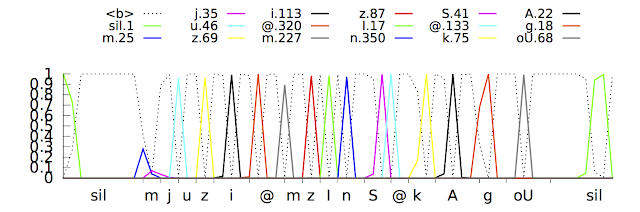
| The CTC recognizer outputs spikes as it identifies various phonetic units (in various colors) in the input speech signal. The x-axis shows the acoustic input timing for phonemes and y-axis shows the posterior probabilities as predicted by the neural network. The dotted line shows where the model chooses not to output a phoneme. |
-
Labels:
- Machine Intelligence
- Product
Other posts of interest
-
April 12, 2024
Contrastive neural audio separation- Machine Intelligence ·
- Sound & Accoustics
-
April 11, 2024
Patchscopes: A unifying framework for inspecting hidden representations of language models- Machine Intelligence ·
- Natural Language Processing ·
- Responsible AI
-
March 28, 2024
AutoBNN: Probabilistic time series forecasting with compositional bayesian neural networks- Algorithms & Theory ·
- Machine Intelligence ·
- Open Source Models & Datasets